---

Interviews

Maintainer - Kevin Naughton Jr.

Translations

• 简体中文

Table of Contents

• YouTube
• Instagram
• Articles
• Online Judges
• Live Coding Practice
• Data Structures
• Algorithms
• Greedy Algorithms
• Bitmasks
• Runtime Analysis
• Video Lectures
• Interview Books
• Computer Science News
• Directory Tree

YouTube

• Kevin Naughton Jr.

Instagram

• Programeme

Articles

• Starting Work

Online Judges

• LeetCode
• Virtual Judge
• CareerCup
• HackerRank
• CodeFights
• Kattis
• HackerEarth
• Codility
• Code Forces
• Code Chef
• Sphere Online Judge - SPOJ
• InterviewBit

Live Coding Practice

• Pramp
• Gainlo
• Refdash
• Interviewing.io

Data Structures

Linked List

• A Linked List is a linear collection of data elements, called nodes, each
  pointing to the next node by means of a pointer. It is a data structure
  consisting of a group of nodes which together represent a sequence.
• Singly-linked list: linked list in which each node points to the next node and the last node points to null
• Doubly-linked list: linked list in which each node has two pointers, p and n, such that p points to the previous node and n points to the next node; the last node’s n pointer points to null
• Circular-linked list: linked list in which each node points to the next node and the last node points back to the first node
• Time Complexity:
  • Access: O(n)
  • Search: O(n)
  • Insert: O(1)
  • Remove: O(1)

Stack

• A Stack is a collection of elements, with two principle operations: push, which adds to the collection, and
  pop, which removes the most recently added element
• Last in, first out data structure (LIFO): the most recently added object is the first to be removed
• Time Complexity:
  • Access: O(n)
  • Search: O(n)
  • Insert: O(1)
  • Remove: O(1)

Queue

• A Queue is a collection of elements, supporting two principle operations: enqueue, which inserts an element
  into the queue, and dequeue, which removes an element from the queue
• First in, first out data structure (FIFO): the oldest added object is the first to be removed
• Time Complexity:
  • Access: O(n)
  • Search: O(n)
  • Insert: O(1)
  • Remove: O(1)

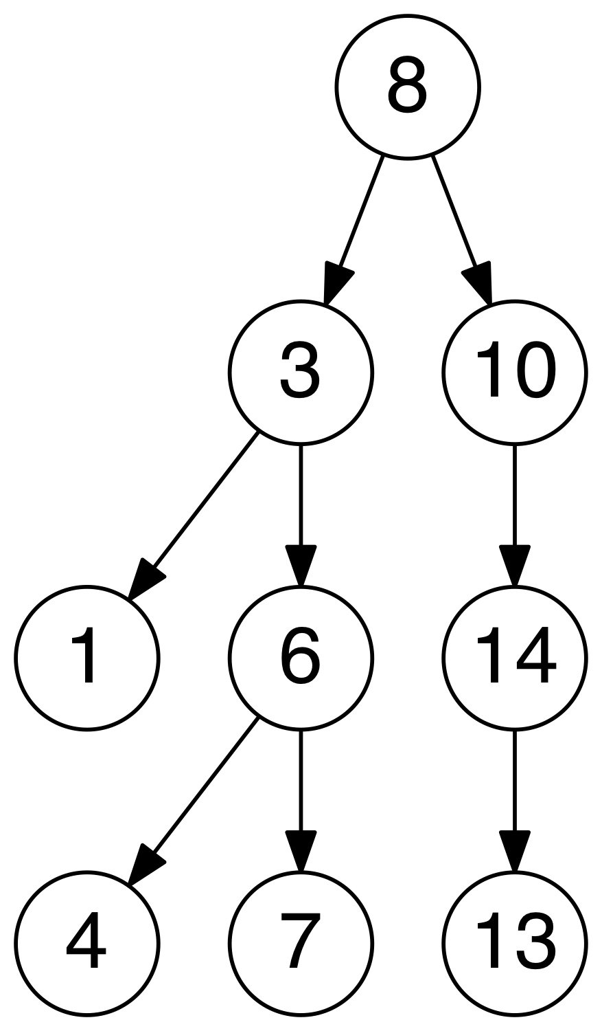
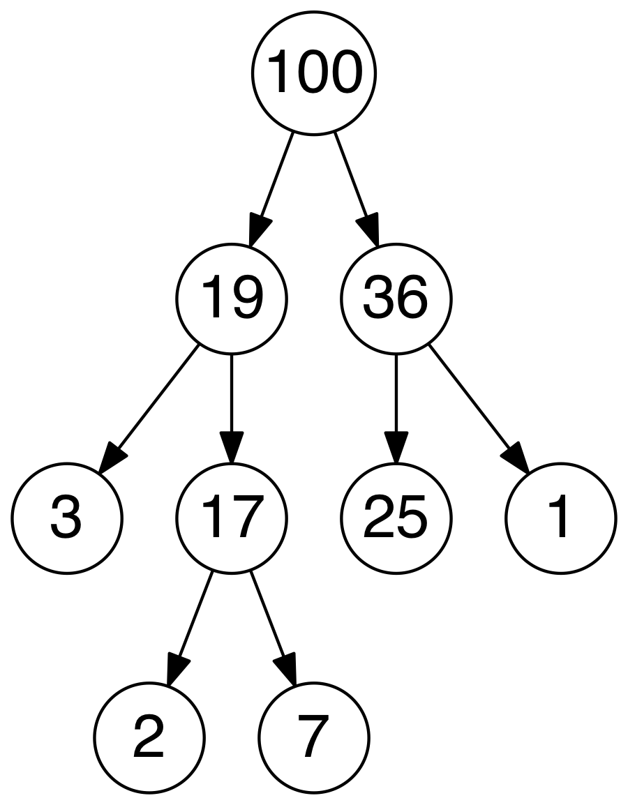
Tree

• A Tree is an undirected, connected, acyclic graph

Binary Tree

• A Binary Tree is a tree data structure in which each node has at most two children, which are referred to as
  the left child and right child
• Full Tree: a tree in which every node has either 0 or 2 children
• Perfect Binary Tree: a binary tree in which all interior nodes have two children and all leave have the same depth
• Complete Tree: a binary tree in which every level except possibly the last is full and all nodes in the last
  level are as far left as possible

Binary Search Tree

• A binary search tree, sometimes called BST, is a type of binary tree which maintains the property that the value in each
  node must be greater than or equal to any value stored in the left sub-tree, and less than or equal to any value stored
  in the right sub-tree
• Time Complexity:
  • Access: O(log(n))
  • Search: O(log(n))
  • Insert: O(log(n))
  • Remove: O(log(n))

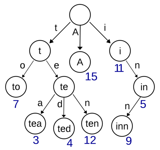
Trie

• A trie, sometimes called a radix or prefix tree, is a kind of search tree that is used to store a dynamic set or associative
  array where the keys are usually Strings. No node in the tree stores the key associated with that node; instead, its position
  in the tree defines the key with which it is associated. All the descendants of a node have a common prefix of the String associated
  with that node, and the root is associated with the empty String.

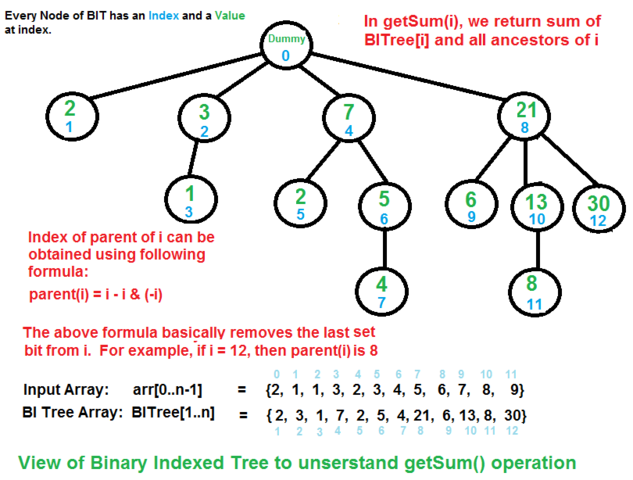
Fenwick Tree

• A Fenwick tree, sometimes called a binary indexed tree, is a tree in concept, but in practice is implemented as an implicit data
  structure using an array. Given an index in the array representing a vertex, the index of a vertex’s parent or child is calculated
  through bitwise operations on the binary representation of its index. Each element of the array contains the pre-calculated sum of
  a range of values, and by combining that sum with additional ranges encountered during an upward traversal to the root, the prefix
  sum is calculated
• Time Complexity:
  • Range Sum: O(log(n))
  • Update: O(log(n))

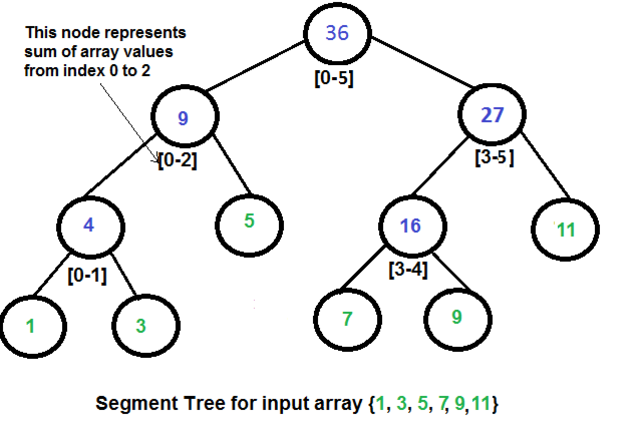
Segment Tree

• A Segment tree, is a tree data structure for storing intervals, or segments. It allows querying which of the stored segments contain
  a given point
• Time Complexity:
  • Range Query: O(log(n))
  • Update: O(log(n))

Heap

• A Heap is a specialized tree based structure data structure that satisfies the heap property: if A is a parent node of
  B, then the key (the value) of node A is ordered with respect to the key of node B with the same ordering applying across the entire heap.
  A heap can be classified further as either a “max heap” or a “min heap”. In a max heap, the keys of parent nodes are always greater
  than or equal to those of the children and the highest key is in the root node. In a min heap, the keys of parent nodes are less than
  or equal to those of the children and the lowest key is in the root node
• Time Complexity:
  • Access Max / Min: O(1)
  • Insert: O(log(n))
  • Remove Max / Min: O(log(n))

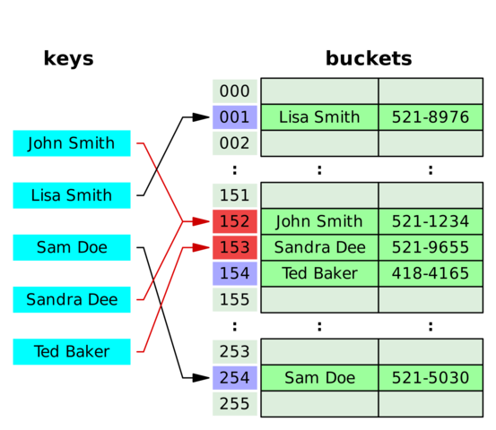
Hashing

• Hashing is used to map data of an arbitrary size to data of a fixed size. The values returned by a hash
  function are called hash values, hash codes, or simply hashes. If two keys map to the same value, a collision occurs
• Hash Map: a hash map is a structure that can map keys to values. A hash map uses a hash function to compute
  an index into an array of buckets or slots, from which the desired value can be found.
• Collision Resolution
• Separate Chaining: in separate chaining, each bucket is independent, and contains a list of entries for each index. The
  time for hash map operations is the time to find the bucket (constant time), plus the time to iterate through the list
• Open Addressing: in open addressing, when a new entry is inserted, the buckets are examined, starting with the
  hashed-to-slot and proceeding in some sequence, until an unoccupied slot is found. The name open addressing refers to
  the fact that the location of an item is not always determined by its hash value

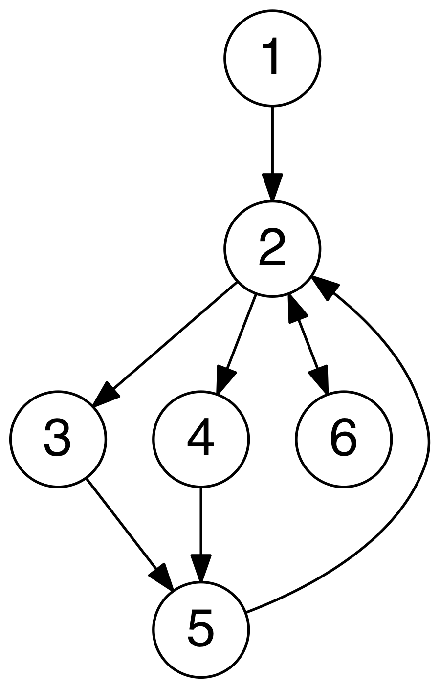
Graph

• A Graph is an ordered pair of G = (V, E) comprising a set V of vertices or nodes together with a set E of edges or arcs,
  which are 2-element subsets of V (i.e. an edge is associated with two vertices, and that association takes the form of the
  unordered pair comprising those two vertices)
• Undirected Graph: a graph in which the adjacency relation is symmetric. So if there exists an edge from node u to node
  v (u -> v), then it is also the case that there exists an edge from node v to node u (v -> u)
• Directed Graph: a graph in which the adjacency relation is not symmetric. So if there exists an edge from node u to node v
  (u -> v), this does not imply that there exists an edge from node v to node u (v -> u)

Algorithms

Sorting

Quicksort

• Stable: No
• Time Complexity:
  • Best Case: O(nlog(n))
  • Worst Case: O(n^2)
  • Average Case: O(nlog(n))

Mergesort

• Mergesort is also a divide and conquer algorithm. It continuously divides an array into two halves, recurses on both the
  left subarray and right subarray and then merges the two sorted halves
• Stable: Yes
• Time Complexity:
  • Best Case: O(nlog(n))
  • Worst Case: O(nlog(n))
  • Average Case: O(nlog(n))

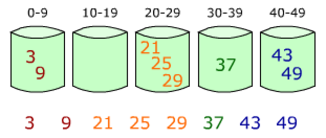
Bucket Sort

• Bucket Sort is a sorting algorithm that works by distributing the elements of an array into a number of buckets. Each bucket
  is then sorted individually, either using a different sorting algorithm, or by recursively applying the bucket sorting algorithm
• Time Complexity:
  • Best Case: Ω(n + k)
  • Worst Case: O(n^2)
  • Average Case:Θ(n + k)

Radix Sort

• Radix Sort is a sorting algorithm that like bucket sort, distributes elements of an array into a number of buckets. However, radix
  sort differs from bucket sort by ‘re-bucketing’ the array after the initial pass as opposed to sorting each bucket and merging
• Time Complexity:
  • Best Case: Ω(nk)
  • Worst Case: O(nk)
  • Average Case: Θ(nk)

Graph Algorithms

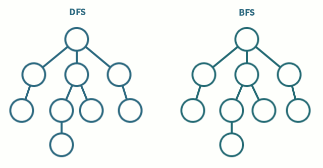
Depth First Search

• Depth First Search is a graph traversal algorithm which explores as far as possible along each branch before backtracking
• Time Complexity: O(|V| + |E|)

Breadth First Search

• Breadth First Search is a graph traversal algorithm which explores the neighbor nodes first, before moving to the next
  level neighbors
• Time Complexity: O(|V| + |E|)

Topological Sort

• Topological Sort is the linear ordering of a directed graph’s nodes such that for every edge from node u to node v, u
  comes before v in the ordering
• Time Complexity: O(|V| + |E|)

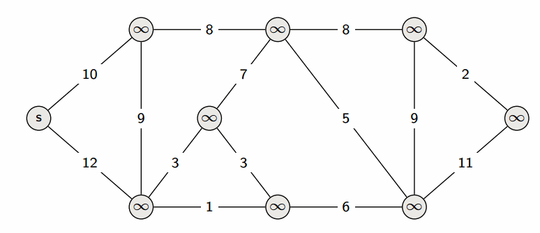
Dijkstra’s Algorithm

• Dijkstra’s Algorithm is an algorithm for finding the shortest path between nodes in a graph
• Time Complexity: O(|V|^2)

Bellman-Ford Algorithm

• Bellman-Ford Algorithm is an algorithm that computes the shortest paths from a single source node to all other nodes in a weighted graph
• Although it is slower than Dijkstra’s, it is more versatile, as it is capable of handling graphs in which some of the edge weights are
  negative numbers
• Time Complexity:
  • Best Case: O(|E|)
  • Worst Case: O(|V||E|)

Floyd-Warshall Algorithm

• Floyd-Warshall Algorithm is an algorithm for finding the shortest paths in a weighted graph with positive or negative edge weights, but
  no negative cycles
• A single execution of the algorithm will find the lengths (summed weights) of the shortest paths between all pairs of nodes
• Time Complexity:
  • Best Case: O(|V|^3)
  • Worst Case: O(|V|^3)
  • Average Case: O(|V|^3)

Prim’s Algorithm

• Prim’s Algorithm is a greedy algorithm that finds a minimum spanning tree for a weighted undirected graph. In other words, Prim’s find a
  subset of edges that forms a tree that includes every node in the graph
• Time Complexity: O(|V|^2)

Kruskal’s Algorithm

• Kruskal’s Algorithm is also a greedy algorithm that finds a minimum spanning tree in a graph. However, in Kruskal’s, the graph does not
  have to be connected
• Time Complexity: O(|E|log|V|)

Greedy Algorithms

• Greedy Algorithms are algorithms that make locally optimal choices at each step in the hope of eventually reaching the globally optimal solution
• Problems must exhibit two properties in order to implement a Greedy solution:
• Optimal Substructure
  • An optimal solution to the problem contains optimal solutions to the given problem’s subproblems
• The Greedy Property
  • An optimal solution is reached by “greedily” choosing the locally optimal choice without ever reconsidering previous choices
• Example - Coin Change
  • Given a target amount V cents and a list of denominations of n coins, i.e. we have coinValue[i] (in cents) for coin types i from [0…n - 1],
    what is the minimum number of coins that we must use to represent amount V? Assume that we have an unlimited supply of coins of any type
  • Coins - Penny (1 cent), Nickel (5 cents), Dime (10 cents), Quarter (25 cents)
  • Assume V = 41. We can use the Greedy algorithm of continuously selecting the largest coin denomination less than or equal to V, subtract that
    coin’s value from V, and repeat.
  • V = 41 | 0 coins used
  • V = 16 | 1 coin used (41 - 25 = 16)
  • V = 6 | 2 coins used (16 - 10 = 6)
  • V = 1 | 3 coins used (6 - 5 = 1)
  • V = 0 | 4 coins used (1 - 1 = 0)
  • Using this algorithm, we arrive at a total of 4 coins which is optimal

Bitmasks

• Bitmasking is a technique used to perform operations at the bit level. Leveraging bitmasks often leads to faster runtime complexity and
  helps limit memory usage
• Test kth bit: s & (1 << k);
• Set kth bit: s |= (1 << k);
• Turn off kth bit: s &= ~(1 << k);
• Toggle kth bit: s ^= (1 << k);
• Multiple by 2ⁿ: s << n;
• Divide by 2ⁿ: s >> n;
• Intersection: s & t;
• Union: s | t;
• Set Subtraction: s & ~t;
• Extract lowest set bit: s & (-s);
• Extract lowest unset bit: ~s & (s + 1);
• Swap Values:

         
  1
  2
  3
  x ^= y;
  y ^= x;
  x ^= y;
  
  

Runtime Analysis

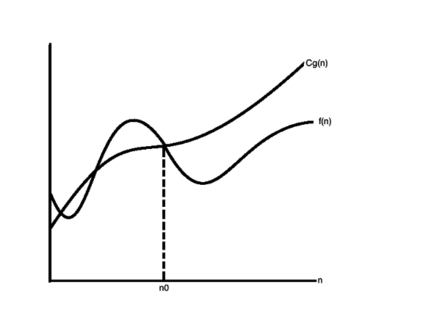
Big O Notation

• Big O Notation is used to describe the upper bound of a particular algorithm. Big O is used to describe worst case scenarios

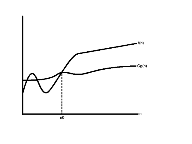
Little O Notation

• Little O Notation is also used to describe an upper bound of a particular algorithm; however, Little O provides a bound
  that is not asymptotically tight

Big Ω Omega Notation

• Big Omega Notation is used to provide an asymptotic lower bound on a particular algorithm

Little ω Omega Notation

• Little Omega Notation is used to provide a lower bound on a particular algorithm that is not asymptotically tight

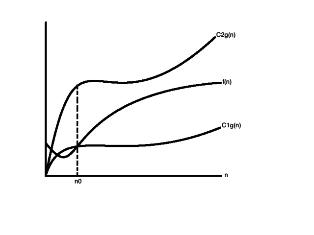
Theta Θ Notation

• Theta Notation is used to provide a bound on a particular algorithm such that it can be “sandwiched” between
  two constants (one for an upper limit and one for a lower limit) for sufficiently large values

Video Lectures

• Data Structures
  • UC Berkeley Data Structures
  • MIT Advanced Data Structures
• Algorithms
  • MIT Introduction to Algorithms
  • MIT Advanced Algorithms
  • UC Berkeley Algorithms

Interview Books

• Competitive Programming 3 - Steven Halim & Felix Halim
• Cracking The Coding Interview - Gayle Laakmann McDowell
• Cracking The PM Interview - Gayle Laakmann McDowell & Jackie Bavaro
• Introduction to Algorithms - Thomas H. Cormen, Charles E. Leiserson, Ronald L. Rivest & Clifford Stein

Computer Science News

• Hacker News
• Lobsters